What Is Attention?

I once overheard an AI researcher—totally real, not made up, lives in Canada—say “Attention Is All You Need.”

So what is attention? And why does this totally real AI researcher want it—and only it?

Let’s find out. This is the first in a trilogy: first the mechanism, then the reach, then the bill.

From Tokens to Embeddings

The Deep Learning book is excellent and roughly the mass of a neutron star in book form, so let’s spare ourselves and open up a real transformer. Since GPUs are now a luxury belief system, we’ll use a model we can still run on a laptop: Phi-3 Mini¹.

Here’s a random sentence:

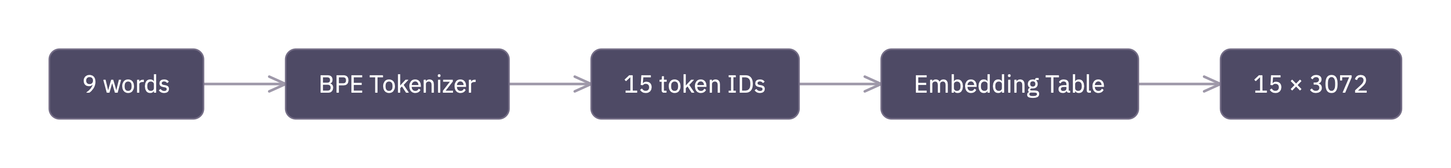
sentence = "Please, for fucks sake, stop buying all the GPUs"

Despite the name, language models can’t read language. They can’t even read words. They get little numbered chunks called tokens and are expected to build syntax, semantics, and civilization from there.

from transformers import AutoTokenizer

tokenizer = AutoTokenizer.from_pretrained("microsoft/Phi-3-mini-4k-instruct")
tokens = tokenizer(sentence, return_tensors="pt")
input_ids = tokens["input_ids"]

Our mini Phi-3 uses a BPE tokenizer²—it learned, during training, which chunks of text appear together often enough to deserve their own ID.³ Common English words usually get a single token each, but punctuation and subwords get their own IDs too. Our nine words are broken up like this:

for id in input_ids[0]:
    print(f"{id.item():>6}  {tokenizer.decode(id)}")

  3529  Please
 29892  ,
   363  for
   285  f
  2707  uck
 29879  s
 16563  sake
 29892  ,
  5040  stop
  1321  bu
  5414  ying
   599  all
   278  the
 22796  GPU
 29879  s

BPE tokenizers are little optimizers: they hand out single IDs only to byte sequences that show up often enough to be worth it. Apparently our training data saw fewer expletive-ridden shopping sprees than our random sentence. So fucks gets split into three tokens and buying into two.

The tokenizer still doesn’t know what words mean. It just notices which byte sequences tend to travel together and rewards the popular ones with their own ID. uck is not just the essence of fuck; it’s also suck, truck, cuck, and muck. The tokenizer is doing compression, not poetry.

Each of these numbers is also a row number in a very large lookup table: 32,064 rows, 3,072 columns. You hand the model a token ID, it slides a 3,072-dimensional vector across the counter. This shady little transaction is called embedding:

from transformers import AutoModelForCausalLM
import torch

model = AutoModelForCausalLM.from_pretrained(
    "microsoft/Phi-3-mini-4k-instruct",
    torch_dtype=torch.float32,
)

embed = model.model.embed_tokens
embedded = embed(input_ids)
print(embedded.shape)

torch.Size([1, 15, 3072])

15 tokens in, 15 vectors out. Each token is now a list of 3,072 floating-point numbers—here are the first 6 dimensions of each:

  Please  [ 0.0020, -0.0303, -0.0236,  0.0737,  0.0199,  0.0378, ...]
       ,  [-0.0225,  0.0012,  0.0293, -0.0002,  0.0032, -0.0028, ...]
     for  [ 0.0613,  0.0065,  0.0231,  0.0359, -0.0234,  0.0060, ...]
       f  [-0.0630,  0.0547,  0.0369,  0.0083, -0.0217,  0.0189, ...]
     uck  [ 0.0201,  0.0625,  0.0182, -0.0302, -0.0099, -0.0564, ...]
       s  [ 0.0034,  0.0181,  0.0250, -0.0032, -0.0074, -0.0040, ...]
    sake  [ 0.0128,  0.0864, -0.0146, -0.0767, -0.0527,  0.0549, ...]
       ,  [-0.0225,  0.0012,  0.0293, -0.0002,  0.0032, -0.0028, ...]
    stop  [ 0.0033,  0.0231,  0.0598,  0.0042,  0.0128,  0.0199, ...]
      bu  [-0.0305,  0.0310,  0.0364,  0.0265, -0.0483,  0.0197, ...]
    ying  [ 0.0061, -0.0654,  0.0276,  0.0608,  0.0047, -0.0091, ...]
     all  [ 0.0056, -0.0208, -0.0283, -0.0227,  0.0383, -0.0381, ...]
     the  [-0.0101,  0.0032, -0.0066, -0.0308,  0.0039,  0.0104, ...]
     GPU  [ 0.0204, -0.0081, -0.0288, -0.0221, -0.0356,  0.0142, ...]
       s  [ 0.0034,  0.0181,  0.0250, -0.0032, -0.0074, -0.0040, ...]

Mostly small numbers, seemingly random. Notice that the two commas have identical vectors, and the two s tokens do too: same token ID, same row in the table, same vector. The embedding stage is a pure lookup. No context. No grammar. No gossip yet.

What are these 3,072 numbers? Not tiny hand-labeled concepts. There is no single dimension for GPU-ness, apology-ness, or interstellar lawless-ness.

Instead, during training, the model learned to arrange tokens in 3,072-dimensional space so that tokens used in similar contexts end up near each other. We can check with cosine similarity — a measure that compares the direction two vectors point, ignoring their length. 1.0 means identical direction; 0.0 means orthogonal:

from torch.nn.functional import cosine_similarity

def tok(word):
    return tokenizer(word, return_tensors="pt", add_special_tokens=False)["input_ids"]

# Same token, same vector
cosine_similarity(embed(tok(",")),    embed(tok(",")))      #  1.00
# Different tokens from our sentence -- basically unrelated
cosine_similarity(embed(tok("stop")), embed(tok("GPU")))    #  0.00
cosine_similarity(embed(tok("Please")), embed(tok("stop"))) #  0.00
# But "GPU" and "CPU" live in similar contexts...
cosine_similarity(embed(tok("GPU")),  embed(tok("CPU")))    #  0.23
cosine_similarity(embed(tok("stop")), embed(tok("halt")))   #  0.18
cosine_similarity(embed(tok("all")),  embed(tok("every")))  #  0.18

stop and GPU are essentially orthogonal. They have nothing to do with each other. But GPU and CPU? stop and halt? The model figured out they’re related without anyone sitting it down and explaining synonyms.⁴

3,072 dimensions is a lot of room. Unrelated tokens can keep their distance; similar ones can cluster together. The individual numbers don’t mean much on their own. The meaning is in the whole encoding.

But we’re still missing the whole point. We looked up each vector independently. The vector for stop is the same whether the sentence says stop buying or stop sign.

The tokens are vectors now, which is progress. But they still haven’t met each other. They have shape, not society.

That’s what attention fixes.

Queries, Keys, Values—and What They Compute

We started with a random sentence, turned it into 15 tokens, and then into 15 vectors. Now what?

Phi-3 stacks 32 transformer layers on top of each other.⁵ Each layer has two departments. First, attention lets tokens exchange information. Then a feed-forward network edits each token privately, door closed, blinds drawn.

We are here for the gossip.

Let’s look inside:

print(len(model.model.layers))
# 32
print(model.model.layers[0])
# Phi3DecoderLayer(
#   (self_attn): Phi3Attention(...)
#   (mlp): Phi3MLP(...)
#   ...
# )

Same structure each time, different learned weights. Let’s grab the first attention layer:

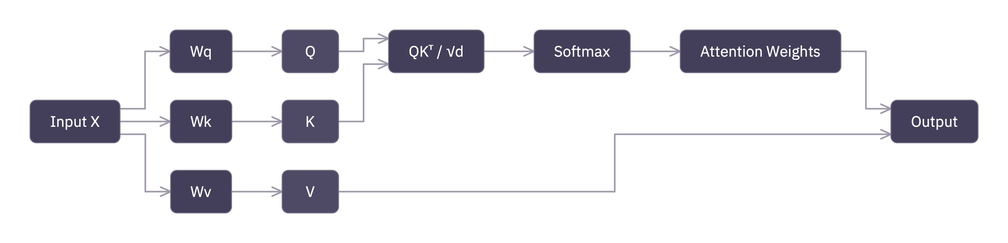
attn = model.model.layers[0].self_attn

This layer has three weight matrices—one each for queries, keys, and values. Each one takes our 3,072-dimensional vectors and produces new 3,072-dimensional vectors:

qkv = attn.qkv_proj(embedded)          # (1, 15, 9216)
Q, K, V = qkv.chunk(3, dim=-1)         # each (1, 15, 3072)

One matrix multiply, three matrices out. Phi-3 fuses the projections for efficiency, then we split the result.⁶

If “query,” “key,” and “value” sound like a database schema from 1998, you’re right. The names are historical. Think filing cabinet.

Splitting into heads

Before we do the actual math, Phi-3 splits each 3,072-dimensional vector into 32 chunks of 96 dimensions. Each chunk is an attention head. Every head gets its own tiny desk and its own opinion about which tokens matter:

def split_heads(x, num_heads=32):
    batch, seq_len, _ = x.shape
    head_dim = x.shape[-1] // num_heads  # 3072 / 32 = 96
    return x.view(batch, seq_len, num_heads, head_dim).transpose(1, 2)

Q = split_heads(Q)  # (1, 32, 15, 96)
K = split_heads(K)  # (1, 32, 15, 96)
V = split_heads(V)  # (1, 32, 15, 96)

Why 32? It’s a design choice: 3,072 dimensions divided by 32 heads gives 96 dimensions per head. More heads means more independent perspectives, but each one has a smaller workspace. The original transformer used 8 heads; larger models use 64 or 128. Phi-3’s designers picked 32.⁷

Each head can learn to care about different relationships. One might track which noun a pronoun refers to. Another might focus on syntax. Others almost certainly do something extremely important that no one has yet named. We concatenate them back together at the end.

The attention computation

OK here it is. The formula the paper title “Attention Is All You Need.” made famous, and the one our totally real AI researcher was so excited about:⁸

$\text{Attention}(Q, K, V) = \text{softmax}\!\left(\frac{QK^\top}{\sqrt{d_k}}\right) V$

Looks intimidating. It isn’t. It’s matrix multiplication in a tie.

Step 1: Score. Compare every query against every key.

scores = torch.matmul(Q, K.transpose(-2, -1))  # (1, 32, 15, 15)

This gives us a 15 × 15 matrix per head. Entry (i, j) is the dot product of token i’s query with token j’s key: a raw score for “how much should token i pay attention to token j?”

That’s the whole query-key story. The query asks. The key answers. Very old-fashioned. Very clerk-and-counter.

Step 2: Scale. Divide by √dₖ to prevent the scores from getting too large:

scores = scores / (96 ** 0.5)  # d_k = 96

This looks like a minor detail. It is not.⁹ Without scaling, the dot products grow with dimension, softmax saturates, gradients vanish, and training falls apart.

One line of code. Entirely load-bearing. Suspiciously so.

Step 3: Mask the future. This is a language model—it predicts the next token. So token i can only look at tokens at positions ≤ i. Peeking ahead would be cheating.¹⁰

n = Q.shape[2]  # number of tokens
mask = torch.triu(torch.ones(n, n, dtype=torch.bool), diagonal=1)
scores = scores.masked_fill(mask, float("-inf"))

Setting future scores to -inf means softmax will give them zero weight. Elegant way to enforce causality. Also an excellent anti-time-travel policy.

Step 4: Normalize. Softmax turns each row into weights that sum to 1. Big scores become big weights, small scores become small weights, −∞ becomes 0. Each token gets a clean “attention budget” of 1.0 to spread across the tokens it can see:

weights = torch.softmax(scores, dim=-1)  # (1, 32, 15, 15)

The first token puts all its weight on itself because there’s nobody else in the room. The last token gets to attend to everyone. It pays to arrive late.

Step 5: Aggregate. Multiply the weights by V:

output = torch.matmul(weights, V)  # (1, 32, 15, 96)

Each token’s output is a weighted average of the value vectors it can see. The Q-K scores decided who to listen to; V provides what they have to say.

That is the retrieval analogy in one line: Q asks, K matches, V delivers.

Putting it back together

The 32 heads get concatenated back into a single 3,072-dimensional vector and passed through one more linear projection:

output = output.transpose(1, 2).contiguous().view(1, 15, 3072)
output = attn.o_proj(output)  # (1, 15, 3072)

Same shape we started with. The sentence went in as 15 vectors of width 3,072 and came out as 15 vectors of width 3,072, but now each one carries information from every earlier token it was allowed to consult. The memo has circulated.

Does this actually work?

We just built attention from scratch. Time to check our homework. The companion package some-attention has a script scripts/post1/attention.py that runs both our manual computation and the model’s own forward pass, then:

assert_close(manual_output, model_output, atol=1e-4, rtol=1e-4)

Instead of dumping a giant tensor, the script prints a quick summary: max error, mean error, and whether the tolerance check passed.

It passes.¹¹

If you followed the code above—project, split, score, scale, mask, softmax, aggregate, merge—congratulations. You understand attention. That is the famous equation. Everything after this is engineering, optimization, or consequences.¹²

Positional Information: RoPE

There’s one glaring problem with what we just built. The attention scores come from QKᵀ, a dot product. Dot products do not care about order. If we shuffled all 15 tokens randomly, the Q, K, and V vectors would be the same, just rearranged, and the attention pattern would come out identical.

That is bad. Stop buying GPUs and GPUs buying stop should not look equally reasonable to anything we’d trust with autocomplete.

Phi-3 fixes this with Rotary Positional Embeddings (RoPE).¹³ The idea is surprisingly physical: before computing QKᵀ, we rotate the Q and K vectors by an angle that depends on position. Token 0 gets a small rotation. Token 14 gets a larger one.

Different positions, different angles, different dot products. Language, as it turns out, was secretly waiting to become trigonometry.

# RoPE is applied to Q and K before the dot product
cos, sin = model.model.rotary_emb(V, position_ids)

# Before RoPE: two tokens with the same embedding
# produce identical Q vectors regardless of position.
# After RoPE: position-dependent rotation makes them differ.
Q_rotated, K_rotated = apply_rotary_pos_emb(Q, K, cos, sin)

Now the dot product between token i’s query and token j’s key depends not just on their content, but on the distance between them. Nearby tokens interact differently than distant ones.

Word order is back. Syntax intact. Civilization preserved.

With RoPE applied, our manual computation matches the model’s output exactly. The companion script scripts/post1/rope.py runs attention with and without RoPE so you can see the difference.

We’re not going deep on RoPE in this series. It’s infrastructure, not the main character.¹⁴ What matters for us is simple: Phi-3 encodes position by rotating Q and K, and the rotation has a base frequency that controls how far the model can “reach.”

That innocent-looking frequency term is the whole bridge to Post 2. If you want a 4k model to pretend it’s a 128k model, this is where the lying starts.

The Quadratic Cost

So how much does all this drama cost?

Look at QKᵀ: every token’s query gets dotted with every token’s key. For n tokens, that’s an n × n matrix. Per head. Per layer. Per forward pass.

The cost is O(n²). Double the sequence length, quadruple the work. This isn’t theoretical. You can feel it in your laptop fan and your life choices:¹⁵

import time

layer = model.model.layers[0]
rotary_emb = model.model.rotary_emb

for n in [128, 256, 512, 1024, 2048]:
    x = torch.randn(1, n, 3072)
    pos_ids = torch.arange(n).unsqueeze(0)
    cos, sin = rotary_emb(x, pos_ids)

    start = time.perf_counter()
    with torch.no_grad():
        layer(x, position_embeddings=(cos, sin))
    elapsed = time.perf_counter() - start

    print(f"n={n:>5}  {elapsed:.4f}s")

Every time we double n, the time roughly quadruples.¹⁶ The companion script scripts/post1/scaling.py runs this more carefully and fits a quadratic, in case you don’t believe your eyes, or your fan noise.

Now do the math for actual use. Our Phi-3 Mini handles up to 4,096 tokens. That’s attention matrices of 4,096 × 4,096: about 16 million entries per head per layer. Not cheap, but still the sort of problem a normal person can ignore.

The same model family has a 128K-context variant. At 128,000 × 128,000, each attention matrix has over 16 billion entries. Same weights. Roughly a thousand times more work. Same equation, much larger filing cabinet, much worse rent.

So the next question is no longer “what is attention?” It’s “how far can this exact mechanism stretch before the math begins misbehaving?”

That is Post 2.